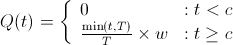
Sequence Locks[1]
05/16/2015Ever been in a situation where you'd give anything just to enforce that threads within the same process would execute through a block of code in a deterministic and configurable ordering? Neither have I, but this post discusses how I'd structure a concurrency mechanism to make that possible.
For a little inspiration, this problem presents itself when you're dealing with many snippets of information (each with a "sequence" number) which need to be interpreted in a specific ordering to tell a coherent story, but are provided to you asynchronously and possibly not in that sequenced ordering. Let's say you are writing a video game client and you receive UDP packets tagged with sequence number and an action, such as
In this case a sequence lock could save Mike's virtual life! In a more generic case with say four threads, here's a diagram explaining how I'd want the sequence lock to work (pardon art skills as always):
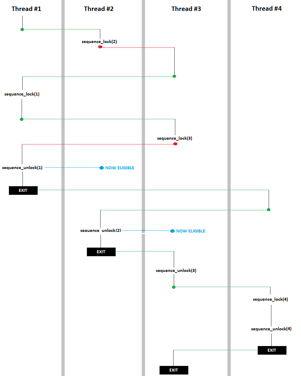
A little explanation on the colored lines:
They key point here being that Thread #1 went through its entire critical section before Thread #2 even entered, and Thread #2 went through its entirely, etc. Also note that no context switch was required for Thread #4's call to sequence_lock(4) as Thread #3 had already unlocked. My task here is implement the functions sequence_lock and sequence_unlock.
In other words, the following should print count from 1 to 300 in order
1 2 3 4 5 6 7 8 9 10 11 12 13 14 15 16 17 18 19 20 21 22 23 24 | public class ShouldPrint1To300InOrder { public static void main(String[] args) { final SequenceLock sequenceLock = new SequenceLock(1l); for(long i = 1; i <= 300; i++) { final long j = i; Thread toRun = new Thread(){ @Override public void run() { try { Thread.sleep((long) (Math.random() * 1000)); } catch(InterruptedException ie) {} sequenceLock.lock(j); System.out.print(j + " "); System.out.flush(); sequenceLock.unlock(j); } }; toRun.start(); } } } |
Here's what I came up with for an implementation of SequenceLock:
1 2 3 4 5 6 7 8 9 10 11 12 13 14 15 16 17 18 19 20 21 22 23 24 25 26 27 28 29 30 31 32 33 34 35 36 37 38 39 40 41 42 43 44 45 46 47 | import com.google.common.collect.Maps; import java.util.Map; /*** * Concurrency variable which can serialize the flow of threads based * on a self-provided sequence number */ public class SequenceLock { //This sequence variable keeps track of who is currently allowed to enter. private volatile Long sequence; private Map<Long, Thread> sequenceToThreadWaiting; public SequenceLock(Long startingSequence) { sequence = startingSequence; sequenceToThreadWaiting = Maps.newConcurrentMap(); } public void lock(Long seq) { synchronized (this) { if(seq.equals(sequence)) { return; } else { sequenceToThreadWaiting.put(seq, Thread.currentThread()); } do { try { this.wait(); } catch (InterruptedException e) { } } while(!seq.equals(sequence)); } } public void unlock(Long seq) { synchronized (this) { if(!seq.equals(sequence)) { throw new IllegalStateException("Called unlock on sequence with " + seq + " but was last locked with " + sequence); } sequenceToThreadWaiting.remove(sequence); sequence++; if(sequenceToThreadWaiting.containsKey(sequence)) { sequenceToThreadWaiting.get(sequence).interrupt(); } } } } |
A few notes on the above
- I am not 100% sure this works - but it seems to pass my tests. If you see something wrong drop me a line!
- One could accomplish this also invoking notifyAll on anybody on the queue for the lock (and not maintaining a map), but then you end up waking up many threads just to put them back to sleep.
- If you use == on the Long objects instead of .equals, you end up with an interesting bug where the lock only works for the first 127 sequence numbers...
- If this was all there was to the SequenceLock class, then you don't need a re-entrant Map, as it is only accessed within synchronized blocks.
[1] Two disclaimers about the name. First, the devised construct is simple enough that it likely has been discussed before (maybe under a different name), but I wasn't able to find anything like this with a quick google search. Second, I just came up with the term "sequence lock," and the proposed device has nothing to do with Wikipedia's SeqLock.
Puzzle from Reddit (link)
04/19/2015My friend linked me a programming puzzle on Reddit and I found it interesting. I didn't get anywhere thinking about it, but I brought it up with my friends and we came up with a neat solution. This post outlines our approach to solving the puzzle (solution below, pardon my artwork as always).
Problem description
As a brief problem description, you are given N input statements giving us the probabilities of various combined events. For instance, in the default example above, the input/output should read:
or, the event "Not A and B" happens with probability 1%. Given many probability assignments like this, the challenge is to find the probability of a target event; in the example above, this is P(A & !B).
Renaming variables for convience in linear algebra
The input statements are not conducive to linear arithmetic manipulation in their undoctored form. For instance, if we are given
we can't combine those equations to get P(A & B), P(A || B), P(A & !B), or really any meaningful combination of the two events; in order to do so we need some quantitative metric of how related A and B are. Notably, however, if we knew that A and B were mutually exclusive, then we can set up linear systems where the probability of one event or another is simply the sum of the two individual probabilities. And that's the first trick - rephrasing the inputs as combinations of mutually exclusive events.
In a universe of N boolean events, there are 2N different, mutually exclusive, outcomes. Specifically, let's label the original events X0, X1, ..., XN-1, and label the entire universe outcomes Y0, Y1, ..., Y2N-1. Let's assume that Y0 corresponds to the specific outcome of
and Y1 corresponds to
and Y2 corresponds to
etc, "incrementing" from "not Xi" to "Xi" like counting in binary.
If we rephrase the problem inputs in this grammar, using Y instead of X, we now get the benefit of knowing that each of our "events" are mutually exclusive; only one element of the Y0 ... Y2N-1 sequence can be true. Because of this, we can add and subtract probabilities and use linear algebraic reasoning. To make this transition, define Y'i as P(Yi) for all i in [0, 2N-1].
Solving the example
Bringing this back to a concrete example, let's start with the example given in the dashed brown box, except let's rename A to be X0 and B to be X1 to be consistent with our naming conventions. We then have
This can be rephrased in the new "Y"-grammar defined above as follows:
Note that X1 actually corresponds the union of the two events, X1 & !X0 with X1 & X0, which is why X1 corresponds to Y1 || Y3. Anyway - we can again rephrase in the new " Y' "-grammar:
As you may have realized, there's an additional equality which goes unsaid - the sum all of everything in the Yi sequence adds up to 1. Recall that the universe is exactly partitioned into the Yi sequence. So, our final linear system is
which we can easily solve with Gaussian row reduction.
Incomplete information
If we take a step back, we solved the example problem by finding the probability of every single true/false assignment to each of the input events. If they've given us enough information, then this is a fine approach. But what if the question was just
In this case, we don't have enough information to solve for all of {Y'0, Y'1, Y'2, Y'3}, but we can still evaluate P(X0), which is Y'2 + Y'3. Rewritten in the " Y' "-grammar,
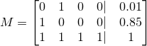
Re-written again as a matrix, M,
This is the second trick of this problem. How can we solve one particular linear combination of variables without solving for all of the variables? The naive Gaussian elimination hinges on being able to solve for all variables and is therefore not a valid solution. One solution is to find some combination of the input expressions which gives you the specific linear combination you're looking for. In the example above, note that
So the problem has changed from solving for Yi to solving for the coefficients of the input equations which you can combine to get the desired linear combination!
To set up the new linear system (which solves for the coefficients of the input equations, not for Yi) we can take the transpose of the unaugmented M matrix, and augment it with the coefficients of the desired linear combination. Neat, right? We are now solving for the coefficients we can use to linearly combine the input equations to get our desired probability. Here is the resultant augmented matrix. The left-side is the transpose of M and the right side is coefficients of Yi representing our desired probability, which is Y2 + Y3.
which, using Gaussian row reduction, we can simplify to
The right-side coefficients here can be used to linearly combine our inputs with our inputs, M to get our desired answer. In matrix form, this is
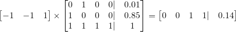
to give our final answer of 0.14 for this problem. And that's all there is to it!
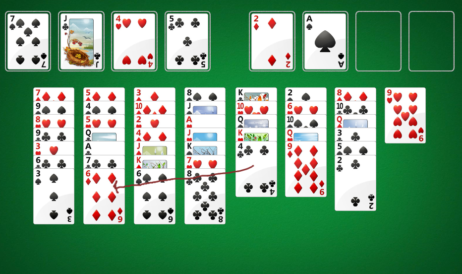
Naive graph-based Freecell solving
07/13/2014One of the Windows-pre-installed games my grandfather plays is Freecell. He's become quite good, but every once in a while he'll dare me to get him out of a particularly stubborn position. I began thinking of ways to- algorithmically solve a Freecell board and reading what others have done on the matter and wrote a Freecell solving app. Nothing was particularly complicated, but I thought it touched upon a few interesting topics and was worth sharing. In this article I'll discuss some of the techniques used to put this together.
Before boring you with the details, however, here's a link for you to play around with the solver.
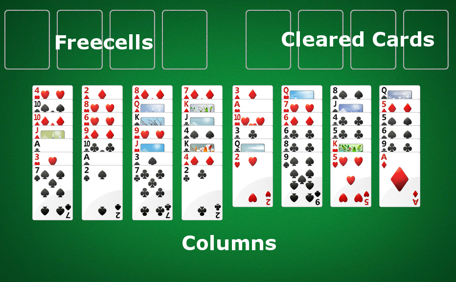
Freecell Solving as Graph Traversal
Where to even begin when trying to code up an algorithm to solve FreeCell? Unlike checkmating an opponent when you have two rooks and king and he only has a king, we can't simply follow a set of rules which will eventually get us to the solution state (whether it be checkmate or moving all of the cards in the foundation cells). Instead, the best I could think of is coming up with a brute-force search of the universe of possible moves.
Imagine we modeled each valid Freecell position as a node, with two nodes being connected if we can move from one to another. This would give us a directed, possibly cyclic, graph. There is only one "completed" node - the one where all of cards have been cleared into the foundation. Representing the problem in this form, we can use any of our favorite graph traversal algorithms to find the solution. Tada!
Pruning and intelligent search
Not so fast - let's do a quick sanity check on the viability of a brute force approach. Let's say there about 8 moves per position (each of the 8 starting columns can move to a Freecell), and say that doing more than 109 operations will take too long. That only gives us log8(109) < 10 moves of depth to search before we run out of operations! If you've ever played Freecell, you'd probably agree that you can't solve many games with 10 moves - for starters there are 52 cards to clear. So it seems though we can't just use a breadth-first-into-oblivion-search or we'd run out of CPU cycles before we found the solution.
Perhaps, however, we could intelligently search only a subset of the graph and still get to the "completed" node. Before we go down that path, it's important to understand that by using heuristics to limit our search space, we are losing our guarantee on finding the shortest solution. Only if our tree was structured better could we find the shortest solution quickly (in polytime) without doing a full BFS-like search. Let's dig into this a bit more. Imagine we're given a constant-time oracle which produces exactly the minimum number of moves to solve the board from any Freecell position - but not the actual solution. Let's call the length of that minimal solution, L. Can you come up with an algorithm to find that minimal solution in polynomial time with respect to L? If you must, the answer is in the footnote.[1]
Unfortunately, I don't know of such a real-life constant time oracle. However, we can use human intuition to build something similar which would give you roughly the number of moves to solve the board from a given position. In fact, the oracle doesn't even need to give you a meaningful number (such as the number of moves required to solve the board) - it can just give you a numeric value monotically increasing (or decreasing) in how good of a position the board is (where a "good" position is one that is close to being solved), and our solver will still find the completed node. This is where we get a chance to put in our "strategies" which will help guide the pruned search to a reasonably short solution.
You can engineer the solver to follow your strategies by having the oracle reward certain pattern and punish others. For instance, we might want the higher ranked cards to be further up in a column, and the 2s, 3s, and 4s to be lower down in a column. We can build the oracle so that it Here are a couple basic strategies that we can hard-code into our solver.
- The more the vacant freecells and vacant columns, the better
- Lower ranked cards are better in the bottom, higher at the top
- The fewer cards remaining in the columns and freecells, the better
Imperfections of a heuristic-based oracle
One problem with an imperfect oracle is that it can lead you uncorrectably astray! Imagine using the algorithm from footnote [1] where at each point you greedily travel to the node with the best oracle score until you've solved the game. With a perfect oracle, the score can never increase from node to another, by construction; there can be no cycles in your solution. At worst, if there is no solution, the score will stay the same and you can therefore detect that there is no solution. However, with an imperfect oracle, the oracle might wrongly suggest you go down one path only to bring you back to where you started - causing an unbreakable cycle. The good news, however, is if you breadth-first-search a few steps in advance and then choose the highest scoring node, as opposed to just choosing the highest scoring immediate neighbor, you can sometimes get over the "humps" caused by a suboptimal oracle. Here is an illustration:
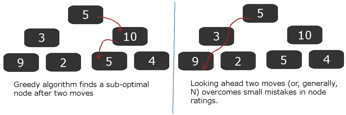
In the diagram above, it should be clear that our heuristic from a node to a "ranking" is a bit flawed - this is what led the greedy algorithm astray. However, real-life Freecell board evaluation algorithms won't be perfect, so tricks like looking ahead a few moves and then choosing the "best" node are helpful. Once you've selected the best leaf node, you only have to remember the path you took to get there. You can forget all the other nodes in the tree and use that memory for further computation.
Move suggestion
Unfortunately even after spending a bit of time on the node evaluation, or "ranking," method my solver would take unusably long to find a solution. I had to come up with another trick. If you're familiar with the rules of Freecell you know that, in the simplest form of the game, you cannot move stacks of cards around between columns. Each turn you can move exactly one card from the columns / freecells to either another column, freecell, or cleared cards. However, some of the Freecell games allow you to move stacks of cards at a time.
It turns out that you can simulate moving a stack of cards at once by a systematic moving of single cards. For instance,
imagine if you had no available free columns, but two available free cells. You can move a stack of up to 3 cards as follows:
So how does this help our solver? It turns out that suggesting "stack moves" as move options (edges in the graph) helps find the solution more quickly because the computer doesn't have to guess all of the single-card moves needed to move a stack, which saves a lot of computation.
As an exercise to the reader, try to prove by induction that you can always move
 cards into a non-empty column, if there are N free cells and K free columns.
Conclusion
Although I don't know of any polynomial-time deterministic freecell solving algorithms, you can use heuristics, move suggestion optimizations, and brute-force search to solve most free cell games. Check out FreeSolved for a free online implementation of the strategies I discussed here. Happy solving.
[1] At each step, evaluate all possible "connected nodes," or neighbors. These represent any possible which can you legally travel to. Choose to move to a node where the "evaluation score" of that node is exactly one less than the current evaluation score. By induction, there must exist at least one such node (if there wasn't a node with score N - 1 neighboring me, then how can I have score N?
Growth Rate, Log Utility, and Kelly Bets
12/06/2012There's a rigged coin with 60% chance of showing heads. You can bet, with 1-1 payout, on heads. You have an initial bank-roll of P. On any given "turn" you can only bet up to the amount of money you currently have. How should you bet over T turns?
This article uses this problem to show that maximizing the asymptotic growth rate and maximizing log utility both result in Kelly betting. It's also true, under asymptotic conditions, that Kelly bets maximize the median fortune of the bettor.[1]
Maximizing expected value
The first thought that comes to mind is to maximize EV of my bankroll over the T turns. If T = 1, EV is maximized by betting the whole bankroll (analysis). Because the coin flips are IID, my decision on each coin flip is unaffected by the past; I should bet the entire bankroll every time!
This strategy does maximize expected bankroll, but most people wouldn't "bet the house" every time because, in all likelihood, you'll be broke after some time.
Maximizing expected utility
As some betting theory suggests, we should be maximizing expected utility, not expected value. In 1738 Daniel Bernoulli
wrote a paper speculating that the marginal utility of money is inversely proportional to the recipient's net worth[2]. In other words,
if a small unit of money brings you the additional happiness of X, then someone who is half as wealthy as you would receive 2X additional happiness from that same sum of money. Mathematically,
 Manipulating this slightly, we see that this is equivalent to the common log-utility function[2]:
Let's use this utility function to determine how much should be bet on one turn. Without loss of generality, assume we have one unit of money.
We are trying to find the optimal bet 0 < b < 1 on this utility function:


In order to find the b which maximizes E[U], find roots of its first derivative while the second derivative is negative.
Finding a root of the first derivative:
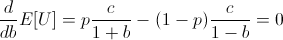


Ensuring that the second derivative is negative there:
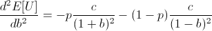
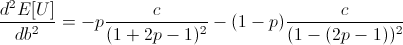
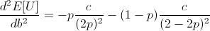
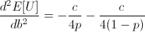
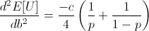 Note that c is the constant from taking the derivative of log(1 + b), and so c is positive.
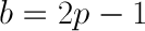
Thus the entire expression is negative, meaning our root at b = 2p - 1 is a local maximum.
Note that c is the constant from taking the derivative of log(1 + b), and so c is positive.
Thus the entire expression is negative, meaning our root at b = 2p - 1 is a local maximum.
Recall that this calculation only solves the "how much should be bet on one turn?" question. Fortunately, because these gambles are IID, we can apply the same result to all subsequent turns, and conclude that for each turn you should bet a fraction of your wealth equivalent to 2p - 1 at each turn. So, to answer our original question if we have a coin with 60% chance of flipping heads, we should bet 20% of our wealth, on heads, every flip.
Maximizing growth rate
Instead of utility, if we maximize the asymptotic rate of asset growth, we arrive at the same result! Formally,
the asymptotic growth rate is defined as
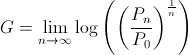
where Pn is the wealth "at time n."[3] In our example, P0 is 1. Now assume that
the bettor is betting some fraction b of his wealth every turn. We can exactly calculate Pn as
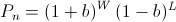
where the bettor wins W times and loses L times. Note that the order of the wins and losses doesn't matter. Simplifying G, we get
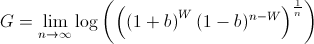
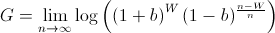
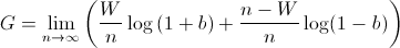
We know that, over time, the bettor will win p amount of the time. Using this, we now must maximize

This is what we want to maximize. But wait a second, this looks an awful lot like the EU of an actor with log utility which we just calculated! In fact, it is!
So maximizing the asymptotic growth rate will have the same result as maximizing EU of a single flip with a log utility function. Thus, if we go through
the math again, we will once again arrive at the conclusion
To further nail in the point, let's consider a different approach. Rewind back to
This is the exact, non-asymptotic amount (not utility) which the bettor will have at the end of W wins and L losses. Let's maximize
this instead using conventional calculus (find root of derivative).


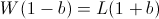

Recall that so far we have not made any asymptotic approximations; the value b described above will always have the highest end balance after W
wins and L losses. As a side note, a negative b value would symbolize taking "the other side of the bet" for the amount abs(b). In order to make further progress, let's now assume that our coin has probability p of flipping heads and the number of trials, n
tends to infinity. We once again have
Maximizing median value
One strategy, which remains largely undiscussed, is to maximize your median wealth value over an indefinitely large sample size. Although I won't go into the math, it also holds that betting 2p - 1 fraction of your bankroll, at all betting turns, maximized the bettor's median fortune over the long run[1].Conclusion
In our simple coin flipping game, both maximizing log utility and asymptotic growth rate yield a betting strategy of betting a fraction of your wealth equal to 2p - 1 on each turn. This result is also achieved by using the Kelly Criterion coined by Kelly in the mid 20th century. The criterion can be expanded and re-calculated whenever the game has payouts other than 1:1, but the essense of the results can be explained in as simple a game as the coin flipping used here. If you're interested in the topic, a few good reads can be found in the footnotes, and in a description of Proebsting's paradox, which surfaces weaknesses of this betting style.[1] This article is meant to be a tip of the iceburg introduction into Kelly betting, but a proof of the median claim can be found here. (S.N. Ethier. 2004).
[2,3] Page two of this paper (MacLean, Thorp, Zhao, Ziemba. 2011).
One last source used was this paper (Stutzer. 2010).
Equity Vesting
10/29/2012Some employers pay employees equity [1] in the company as part of their compensation. And just like how you don't get your entire annual salary in the first pay check, you don't receive all of your equity on the first day. This article does some analysis on the equity vesting process.
Employees
We'll simplify our analysis and assume that employees are rational actors with common utility curves that get value only out of money. In short, this means that employees always prefer more money to less money, and receive strictly decreasing marginal happiness on each additional dollar as they get richer.
We'll also assume that our employee is looking to maximize utility for some arbitrary time, pick two years from now[2]. In the meanwhile employees are free to move around companies at their will.
Companies
Assume companies pay employees in salary and equity. The value of paid salary in two years has low variance, but the value of equity two years from now is less predictable especially for unestablished companies.
Companies give employees equity in the company according to a vesting schedule. A simple linear equity vest gives the employee equity linearly proportional to the amount of time they've worked at the company until they've vested all of their equity. For example if an employee is granted 20 equity units over 4 years with a linear vest, he gets 5 units after the first year, 10 after the second, etc. until the end of the fourth year at which point he recieves no more equity.
Startup Example
Let's consider our employee Bob who wants to work at a startup company. He has a common utility curve, such as

Bob has two years to maximize his expected utility. Let's simplify the world and assume the only options Bob has during this time are to work at either Startup A or Startup B.
Both startups give equity that vests linearly over 2 years and have an independent 5% chance of "making it,"[3] and a majority chance of sizzling out with worthless equity. The equity values in the table below, in the same units as salary, are assuming the company "makes it."
| Equity earned after t years | Salary earned after t years | |
|---|---|---|
| Startup A | 1000t units | 5t units |
| Startup B | 900t units | 4t units |
Let t be the time, in years, Bob spends working for Startup A; (2-t) is the time he works for Startup B. From the looks of it, Bob should work for Startup A for all two years. The only two options are A and B, and he should never be working for the latter because A seems more lucrative. Right? Let's see.
| Who makes it? | Chance | Monetary value | Simplified payout |
|---|---|---|---|
| A, B | 0.25% | t(1000+5)+(2-t)(900+4) | 101t+1808 |
| A | 4.75% | t(1000+5)+(2-t)(0+4) | 1001t+8 |
| B | 4.75% | t(0+5)+(2-t)(900+4) | -899t+1808 |
| Neither | 90.25% | t(0+5)+(2-t)(0+4) | t+8 |
Let's do some expected utility math. Recall that t is the time Bob works for Startup A. Bob expects his utility to be
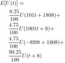
This turns into a simple optimization problem, trying to maximize the above expected utility where
After doing some math (finding roots of derivative of expected utility), we see that expected utility is highest where

In English, this means that Bob should leave the more seemingly lucrative Startup A for a worse opportunity around 15 months into the job.
What may be even more surprising is the following Wolfram Alpha chart with expected utility on the Y Axis and time spent working for Startup A, in years, on the X Axis:
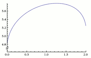
Above we can see that leaving the "better job" after 6, 12, or 18 months are all better options than staying for two years!
The problem with linear vesting
Woah! The payout schedules (under all of these assumptions) actually encourage a rational actor with a common utility curve to leave for a "worse" startup!
This dilemma is the reason why, more simply put, most people prefer a 2% chance shot at $1 million rather than a 1% shot at $2 million. This encourages jumping ships.
The odd thing here is that startup companies often choose a vesting schedule (such as a linear) that causes this dilemma, when they really want the employee to stay for longer!
Mitigating this effect
First off, because of all the assumptions made, our analysis isn't a great correlation to the real world. Nonetheless, the fundamental idea that common utility curves imply risk-averse "hedging" behaviour is something that we have to learn to deal with in compensation packages.
Cliffs
A popular way to mitigate this effect is to impose a cliff on the equity vesting. A linear vest of w equity units over period T with no cliff (of an employee that's worked for t time) has
In English, this means that your ownership of the company increases linearly with time until you you've worked for T time at which point you've received all of your equity. A cliff up until time c means that should you work for less than c time units, you receive no equity. So,
Cliffs discourage employees from leaving before the cliff period, but don't solve the underlying asymmetry between payout and utility. If both Startup A and B had imposed a 1 year cliff, Bob would've still worked for Startup A for about 15 months and left to work for Startup B!
Non-linear vesting
Let t be the time the employee has worked for a company. Our linear vesting schedules can be expressed as

Instead consider the following vesting schedules, which promise the exact same amount of equity after 2 years:
Instead if we re-calculate Bob's optimal moves, we'll see that he should (this time around), work for Startup A for the entire two years. This is because the payout schedule is slower than his utility curve is conservative; Bob doesn't start earning any real equity unless he hangs around which more than accounts for his desire to hedge his bets by jumping ships.
In real life, higher order polynomial equity vesting schedules may be too "complicated", so a more practical solution is delayed additional grants. Assume that startups A and B instead offered Bob one third as much equity in his initial grant, but then gave him two additional equity grants one year apart after he joined. All equity grants vest over two years, with the first one cliffed. His payout would like
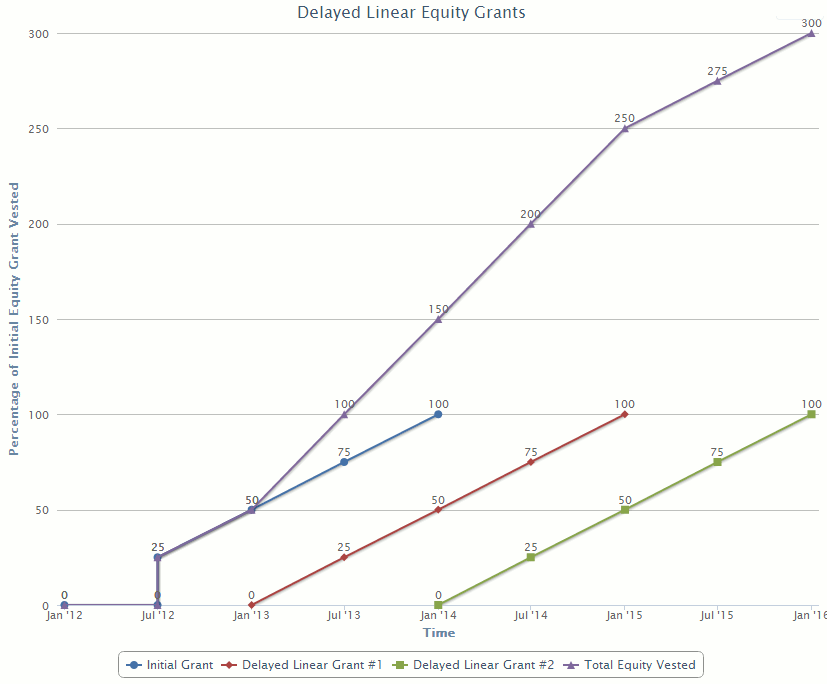
This payout, just like higher order polynomial schedules, maintains the desirable positive second derivative in the beginning which helps mitigate risk aversion.
Conclusion
Unestablished companies generally are subject to having a high variance on equity worth. The linear equity vesting schedule, even with a cliff, may not be the best from a rational perspective.
[1] For the purposes of this article, equity can be anything which rises in monetary value as the company does, like shares (linear value correlation) or options.
[2] This isn't a great approximation but will suffice for the analysis. It might make more sense to assume employees are maximizing the overall utility over time with various weights given to different times. Specifically, employees are looking to optimize:
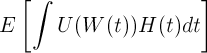
where U(w) is the utility for a given wealth, W(t) is the wealth at time t, and H(t) is how much the actor weights happiness at that point in time. For an actor who is optimizing to have a great time in his 30s, H(t) may look like
[3] I actually believe the entire world is predictable, but since I can't even tell you what I'm going to have for lunch tomorrow, let alone what companies are going to be worth, I'll fall back on random modeling.
Books I like
10/01/2012With indexed, searchable, up-to-date, dynamic resources at our disposal I find books becoming less and less useful. Good books, however, are able to present a lot of relevant information with little noise and a coherent structure; this can be tough to find online without a lot of searching. I found these ones totally worth it:
Computer Systems: A programmer's perspective
Great introduction to systems. The only thing is that I might be biased as I taught with the authors and maybe share their way of explaining things. Topics include:
- Data representation
- x86(_64), ELF, stack, & execution
- VM, translations, caches
- Processes, threads, signals
- System I/O
- Intro to network programming
- Intro to concurrency
There is a newer version, and I'd think that it's better, but I learned from this one haven't used the newer one. And don't worry, I wasn't paid to say this and none of these links are give me referral money.
Introduction to Algorithms
Covers undergraduate algorithms, assumes some knowledge of common structures and basic strategies. Maybe it just happens to be what employers look for in CMU students, but this book is excellent for CS interview preparation coming out of school.
I also had the first-class information in this book presented to me by one of my all-time favorite teachers, Avrim Blum.
There is a newer version of this book as well, but I haven't used it.
Databases and Transaction Processing
I never took a formal course on database internals in school (c'mon, MIS doesn't count), but I feel like I've got the gist of it thanks to this guide.
I think the book is meant for a variety of audiences and so doesn't assume much prior knowledge at all. Consequently it starts out pretty slowly, but definitely gets into hard tech eventually.
CSS Mastery

It's tough to be in tech these days and fully avoid web frontend work. And at this point you've probably noticed that I'm no master of CSS, but quite the opposite. To make matters worse I have very little design talent or experience. But I've tried to embrace the beast and my knowledge about CSS, web layout, etc. is probably an even split between this book, www.w3schools.com, and the rest of the internet.
There is a newer version of this book as well, but I haven't used it.
Thanks for reading!
Hopefully some of these come in handy to you. If you know of any good reads in other subjects (AI/ML, Stats, Networks, etc.) let me know!
How much would you bet?
08/09/2012When you want to know how confident someone is, you might ask them "How much would you bet?" This article discusses what it means to be willing to bet X on something.[1]
Let's define the event A as some occurrence which you might bet on. For instance, A might be the event of the Steelers winning a playoff game. We'll refer to P(A) as the perceived chance that A happens.
Rationality
Let's define a rational actor as a decision maker who always chooses the path with the highest expected happiness, or expected utility. In the case of betting, a rational actor will take a bet only if he expects it to leave him in a state of higher utility than refusing the bet. Utility can be expressed as a function of the state of the actor's life; in the real world, these factors may include personal net worth, satisfaction with family life, career, etc. Note that an actor can derive happiness from making others happy, so rational actors aren't always "selfish" in the conventional sense[2].
Our example
For simplicity, let's assume our rational actor derives strictly increasing happiness off of only his own bank balance, P with initial value P0.
Our example will be the following question: "How much would you bet that the result of a fair dice roll is greater than 2?"
Analysis
A is the event of rolling a 3 - 6, and so by elementary statistics

Assume now that the actor was trying to bet some value b such that his expected bank balance is maximized. With some math,
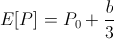 it follows that the actor's bank balance is maximized when he bets everything! Moreover, we would reach the same conclusion for any event A which has even a 51% of happening.
But most people wouldn't bet their entire bank balance on something as risky as 51% because they are trying to maximize utility, not bank balance.
It's not too hard to see that if utility is positively linear in bank balance,
we arrive at the same result of maximizing the amount bet.
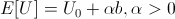
Utility functions
Why did maximizing bank balance yield the same result as maximizing utility of a function linear with bank balance? To answer this, first define two utility functions as equivalent if a rational actor following one utility function would always make the same choice as an actor following the other. It turns out that utility functions which are positive linear transformations of each other are equivalent[3].
However, utility functions are generally non-linear in wealth and can result in more interesting solutions.
Two properties of common utility functions are that they are strictly increasing in wealth (non-satiability), and that they have diminishing returns over wealth. Formally,
For our basic example, let's take the following utility function (satisfying above properties):

Back to original problem: How much would you bet that the result of a fair dice roll is greater than 2? Let's assume that our rational actor starts with P0 = 100. Let's start by calculating some expected utilities:
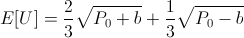
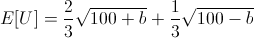
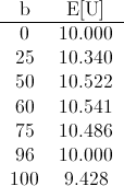
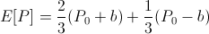
Here we can see that our rational actor under this utility curve would actually refuse a "bet-it-all" on the dice roll as he expects it will leave him in a lesser utility state even though there is a two-thirds chance of winning.
One interesting thing here is that the actor's expected utility is maximized if he bets b = 60[4], but any bet 0 < b < 96 leaves him in a higher utility than no bet at all! So the answer to the question, for this actor with initial wealth 100 and square root utility curve, would be that he's willing to bet up to 96 units but prefers to bet exactly 60 units.
So back to square one. The layman phrase "How much would you bet?" actually could take quite some effort to answer rationally. The methodology, or thinking, used to reason here can be applied to arrive at a variety of conclusions. Try deriving the following truths (ordered in increasing difficulty) on your own:
- 1) In our example above, a wealthier rational actor would have been willing to bet more than 96 units.
- 2) With "common" utility functions, a rational actor wouldn't be willing to bet anything on a 50-50 bet.
- 3) Two utility functions, U0, U1, are equivalent if and only if
[1] This article is a tip-of-the-iceberg introduction to utility theory. This paper by John Norstad is a very enlightening, easy read I thoroughly enjoyed.
[2] For instance, consider the case where my happiness function is increasing in both my bank balance (with diminishing returns) and my sister's bank balance (with diminishing returns). It's possible that if I strike it rich, it would make me happier to give a chunk of money to my sister rather than keep it; even though this appears to be a selfless choice, this would be the decision of the self-serving rational actor.
[3] Utility theory paper
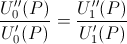
[4] As an exercise to the reader, find the maximum expected utility by symbolically solving for roots of the first derivative of the utility expectation function with respect to the bet amount.
Randomness
07/05/2012This post is about thoughts I had on randomness and indeterminism. Inspired by "God doesn't play dice" - Einstein
School
In school, I often solved problems assuming that certain events was intrinsically indeterminable. In signal processing you may assume there is some unknown noise, in economics you plan for uncertainty of markets, and in stats classes you begin with the assumption random variables exist and take on different values with various likelihoods. We're then taught to manipulate these objects, defining and deriving different properties of random variables. Finally, we use this knowledge in "practical" applications like finance or engineering.
All this time I never questioned the existence of incalculable events. After all, consider a dice roll or a coin flip. In class these were quintessential examples of real world randomness.

"Randomness" because of Information Incompleteness
If we look more closely at our coin, I argue that we only model a coin flip as random because we can't calculate it exactly. Similarly, we only model a dice roll as random because we can't calculate all the rotations and collisions associate with a dice roll. There is in fact nothing random at all about either a dice roll or a coin flip. If your statistics exam gave you more details on exactly how the coin was tossed or dice was rolled, you could solve the problem without any randomness. But then it would probably be a physics exam.
In less words, we fall back on modeling outcomes as random whenever we have incomplete information.
Living by the beach
To drive home the point, imagine if we didn't understand the concept of buoyancy. We live by the ocean, and some objects we throw in sink and some float. We can't actually figure out why, so we run 1000 experiments. In each experiment we throw in some object into the water and note down whether it floats or sinks. At the end of the this very complicated experiment, we come to the conclusion that floating is a Bernoulli random variable with 74.3% of objects sinking and 25.7% floating. Wow! Sounds right to me! In actuality, if we just had a better understanding of the world, we would be able to exactly calculate whether an object will sink or float and remove randomness entirely. Same goes for coin tosses, dice rolls, the weather tomorrow, and ... humans.
Indeterminism and lack of free will
Here's where it starts getting controversial. Most people would agree that[1], if you had a computer and physics genius, you could exactly calculate how everything will unfold in a Rube Goldberg machine.

Cartoon of a complicated Goldberg machine
Now, if we had a electro-chemistry/biology/neuroscience genius and a computer, can we calculate exactly how a living cell will behave? Or how about a human? The same type of particles which make up a mechanical Rube Goldberg make up biological humans. If the behavior of the particles of the former can be predicted, why can't humans? Is consciousness and thinking anything more than the effects of neurons firing? A rolling ball which triggers a gear turning is analogous to a neuron firing triggering a muscle flex. Remember that we're not actually concerned about actually predicting human behavior, but rather about knowing whether or not it is predictable at all.
From this, we can look at life as a whole as a big Rube Goldberg which is just unfolding itself; everything is pre-determined and just waiting to happen. Furthermore, if our model of physics (how the world works) was perfect, it would even be calculable!
Take away
Outcomes are often modeled as random because of incomplete information, not because of genuine randomness. It is within the realm of possibility that all outcomes are calculable with an accurate enough model of the world, eliminating the need for random modeling.
Does this mean we should stop teaching how to find the standard deviation of a random variable? Probably not. Random models are a great practical backup plan that have provided tremendous value. So kids, until you come up with an exact deterministic calculus for all outcomes, you can't use this as an excuse for unfinished stat homework.
[1] From my embarrassingly little knowledge of Quantum Mechanics, the latest theories say that there is in fact genuine randomness and incalculability in how matter behaves at this level. If this is true, then randomness has been introduced into the world and so the whole determinism argument falls apart. However, if the current theory simply introduces randomness to satisfy discrepancies between the theory and observed experiments and there exists an accurate deterministic theory, then determinism still holds.